Stencil Optimization for Deferred Lights Without Depth Clamp

Using two sided stencil volumes to improve fill rate with deferred lights is not new; I'll write more if anyone wants, but this is all stuff I got off of the interwebs.  The high level summary:

• To save fill rate when drawing deferred lights, we want to draw a geometric shape to the screen that covers as few pixels as possible - preferably only the ones that will be lit.
• Typically this is done using either a billboard or a bounding volume around the light.  X-Plane 10 uses this second option, using a cube for omnidirectional lights and a quad pyramid for directional lights. (This is a trade-off of bounding volume accuracy for vertex count.)
• If we have manifold bounding volumes, we can select only the fragments inside the volumes using a standard two-sided stenciling trick: we set the back face stencil mode to increment on depth fail and the front face stencil mode to decrement on depth fail - both with wrapping.  The result is that only screen-space pixels that contain geometry inside the volume (causing a depth fail on the back face but not the front face) have an odd number of selections.
• Once we have our stencil buffer, we can simply render our manifold volumes with stencil test to discard fragments when our more expensive lighting shader is bound.

So far, all standard.  Now what happens when the near and far clip planes interfere with our bounding volume?

• If the front of the volume intersects the near clip plane, that's no problem - the front facing geometry isn't drawn, but since there was no geometry in front of our light volume (how could there be - it would also be on the wrong side of the near clip plane too) this is okay.
• We need to render the back face only of our volume to correctly rasterize the entire light.  If we rasterize the front, we'll draw nothing when the camera is inside the light volume, which is bad.  (This need to handle being inside the shadow volume gracefully is why Carmack's Reverse is useful.)

If the back of the volume intersects the far clip plane, we have a bunch of problems though.

• When drawing the actual light volume, we're going to lose a bunch of our screen-space coverage, and the light will be missing.
• When we're using stenciling, the increment/decrement pattern will be broken.  If we have geometry in front of the entire light, it will end up off-by-one in its surface count.  This in turn can interfere with other lights that cover the same screen space.

This last case shows up as a really weird looking bug in X-Plane: when the landing light is on and pokes out the far clip plane, we can get a cut-out that removes other area lights that cover the screen-space intersection of the landing light volume and the far clip plane.

The simple solution is obvous: use GL_depth_clamp to the near and far clip planes instead of clipping.  But what if you don't have this extension?

In these pictures, we are seeing only a close rendering of the P180 - the far clip plane is just off the end of the airplane.  The red cone extending from the tail is the pyramid light volume for the tail light that is shining out from the tail - it illuminates the top of the plane.

In the three pictures the far clip plane is progressively moved farther away.  The lighter colored square is the missing geometry - since the pyramid is clipped, you're seeing only the top and sides of the pyramid but not the base.  This is the area that will not be correctly stencil counted or rasterized.

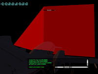
Here we can see why this is a problem.  Note the vertical line where the back face is missing.  When we actually rasterize, we don't get any light spill - the result is a vertical clip in our light, visible on the top of the fuselage.





If depth clamp isn't available, one alternative is to restrict the Z position of each bounding volume vertex in clip space.  This can be done in the vertex shader with something like:

gl_Position.z = clamp(gl_Position.z, gl_Position.w,-gl_Position.w);

(W tends to negative for standard glFrustum matrices.)

What's nice about this hack is that it is entirely in vertex shader, which means that we don't do anything that could inhibit the GPU's ability to do early or optimized Z culling.

The actual screen-space position of the view volume does not change.  This is because the position edit is done in clip space, and clip space is orthographic - X and Y turn into raster positions and Z into a depth position.  The "perspective" is created by dividing X and Y by W - we're free to completely whack Z without deforming the geometry as long as we are post-frustum-transform.

Wel, not completely free.  There is one hitch: the actual Z test is no longer correct.  Observe these two pictures:

 In the first picture, we see the correct Z intersection of the view volume with the fuselage.  (This picture is normal rendering with a close far clip plane, hence the lack of a pyramid back.)  The area of the fuselage that is not red is outside the light bounding volume, and there is just therefore just no need to shade it.

Now look at the second picture - this is with Z clamping in the vertex shader.  Because the Z position has been clamped pre-interpolation, the Z fragment positions of any face that partly extended outside the clip planes will be wrong!

In the picture we see this in the form of incorrect volume intersection.  Because the far end of the pyramid has been moved closer to us (to keep it inside the far clip plane) the fragments of the entire pyramid are too close to us - almost like a poor-man's polygon offset . The result is that more of the fuselage has turned red - that is, the Z test is wrong.  The actual Z error will sometimes reject pixels and sometimes accept pixels, depending on the precise interaction of the view volume and the clip planes.

The net result is this: we can hack the Z coordinate in the vertex shader to guarantee complete one-sided rasterization of our view volume even with tight clip planes and no depth clamp, but we cannot combine this hack with a stencil test because the stencil test uses depth fail and our depth results are wrong.

Thus the production path for X-Plane is this:

• In the "big" world we use two-sided stenciling.
• In the "small" world if we have depth clamp we use two-sided stenciling and depth clamp.
• In the "small" world if we don't have depth clamp we use vertex-shader clamping and skip stenciling.

*This is actually a real question for X-Plane 10 running on OS X 10.6.8; the ATI drivers don't support the extension and in X-Plane we don't want to push out the far clip plane for the in-cockpit render.*  Is there any other way?* The truth is, the motivation to keep the far clip plane close is mostly a software-organizational one - the sim could run with a farther far clip plane but a lot of code uses the real view frustum and would have to be special-cased to maintain efficiency.

Bezier Curve Optimization

I've been meaning to write up a few notes about how we turn OSM vector data into bezier curves for X-Plane.  The code is all open source - look in the scenery tools web code browser at NetPlacement.cpp and BezierApprox.cpp for the code.

First, a few basics:

• OSM vector data comes as a polyline data - that is, each road is a series of points connected by straight line segments.  There are a lot of points - sometimes every few meters along a road.
• X-Plane 10 uses piece-wise bezier curves, meaning a road is a string of end-to-end bezier curves.  Each curve can be a line segment, quadratic, or cubic bezier curver, but not anything of higher degree.  
• The representation in X-Plane for the piece-wise bezier curves is a list of "tagged" points, where the tag defines whether a point is a piece-wise curve end-point or control point.  Semantically, the two end points must not be control points (must not be tagged) and we can never have more than two consecutive control points (because that would define a higher-order bezier).
• There is no requirement that the curve be smooth - we can create a sharp corner at any non-control point, even between two bezier curves.

Both OSM and X-Plane's road system have network topology, but for the purpose of converting a polyline to a piece-wise bezier curve we care only about a single road between junctions - that is, a "curve" in topology-terms.

We divide the problem into two parts: converting the polyline to a piece-wise bezier curve and optimizing that bezier curve to reduce point count.

To build the initial beziers we take an idea from ATI's PN-Triangles paper. The basic idea from the paper is this: if we have a poly-line (or triangle mesh) approximation of a curved surface, we can estimate the tangents at the vertices by averaging the direction of all incident linear components.  With the tangents at the vertices, we can then construct a bezier surface through that tangent (because a bezier curve's tangent at its end point runs toward the next control point) and use that to "round out" the mesh.

The idea is actually a lot easier to understand for polylines, where the dimensionality is lower.  For each vertex in our road, we'll find the "average" direction of the road (the tangent line) at that vertex based on the two segments coming into that vertex.  The bezier control points adjacent to the vertex must run along that tangent line; we can then adjust the distance of the control points from the end point to control the amount of "bulge".

We start with a poly-line.

We calculate the tangents at each vertex.

We place bezier control points along the tangents at fixed fractional lengths.

The result is a smooth piece-wise approximation through every point.

PN triangles tends to make meshes "bulge", because a curve around a convex hull always extends outward.  You can see the same look in our interpolation.  This is good for on-ramps but actually looks quite bad for a straight-away road - the road "bulges out" when the curve ends.

To address this, we categorize a road as "straight" if the road is long enough that if we built a curve out of it, the radius of that curve would be larger than a constant value.  (We pick different constants for different types of roads.)  In other words, if two highway segments are each 1 km long and they meet at a 3 degree angle, we do not assume it is part of an arc with a 19 km radius - we assume that most of the 1 km road are straight, with a small curve (of much smaller radius) at the end.  For any given point, we can decide whether either one or both of the two adjoining line segments is "straight" or should be entirely curved.  We then form five cases:

1. If two segments come together at a very sharp angle, we simply keep the sharp angle.  We assume that if the data had this sharp angle in the original vector data (which is quite highly noded) then there really is some kind of sharp corner.
2. If the two segments come together at a very shallow angle, we simply keep the corner, because who cares.  This case matters when we have a very tiny angle (e.g. 0.25 degrees) but very long line segments, such that removing the tiny angle would cause significant change in the vector position due to the long "arm" and not the steep angle.  We trust that for our app the tiny curve isn't going to be visible.
3. If the two segments are both curved, we use the PN-triangle-style tangents as usual.
4. If one of the segments is curved and one is straight, the tangent at the point comes from the straight curve.  This takes the "bulge" out of the beginning and ending of our curves by ensuring that the curve ends by heading "into" the straight-away.
5. If both segments are straight, we need to round the corner on the inside.  We do this by pulling back the corner along both curves and using the original point as a quadratic bezier control point.

One note about cases 2 and 5: if you pull back a vertex proportional to the angle of the vertex, then very small angles can result in very small pull-backs, resulting in a very short curve.  In the case of X-Plane, we want to ensure that there is a minimum distance between points (so that rounding errors in the DSF encode don't give us colocated points); this means that the minimum angle for case 2 has to be large enough to prevent a "tiny curve" in case 5.

The five curve cases, illustrated.

With these five curve cases we get pretty good looking curved roads.  But our point gets out of control - at a minimum we've kept every original point, and on top of that we've added one or two bezier contrl points per segment.

What we need to do is generalize our curves.  Again, the PN-triangles observation can help us.  If we want to replace two piece-wise bezier curves with a single one, we know this: the tangent at the end of the curves can't change.  This means that the two control points of the approximate curve must be colinear with the control points of the original curve ends and the original curve ends itself.

So what?  Well, if we can only move the control points "in and out" then there are really only two scalar variables for all possible approximations: how much to scale the control handles at the start and end.  And that's something we can check with brute force!

Below is the basic step to approximating a piece-wise bezier curve with two pieces as a single cubic bezier.

We start with a piece-wise bezier with nodes and control points.

For each range of curves that we will simplify, we "push" the outermost control points along the tangent vector by an arbitrary scaling factor.

The resulting curve will be close, but not quite the same as the original.

The original also looks "reasonable" on its own - that is, the approximations tend to have good curvature characteristics.

To find the approximate curve, we simply "search" a whole range of scalar values by trying them and measuring curve error.  In the scenery tools code, we do a two-step search, refining the scalars around the values of least error.  The initial values are picked experimentally; it's almost certainly possible to do a better job of guessing scalar values but I haven't had time to research it more.

To measure the error we approximate the bezier with polylines (e.g. we turn each individual bezier into a poly-line of N segments) and then compare the polylines.  The polyline comparison is the variance of the distances of each point in one polyline to the other. (in other words, we treat one polyline as a point set and take the variance of the distance-to-polyline of each point).  This is similar to the Hausdorff distance with two key differences:

• Because we are taking variance and not a minimum error, we can't use our previous minimum distance from a point to a line segment to limit our spatial searches.  (See below.)  Instead, we pick some large distance beyond which the curves are too different and we use that to limit.  For low maximum acceptable errors this gives us good performance.
• Since the variance depends on all points and not just the worst one, we can rank multiple approximations - that is, generally better approximations score quite a bit higher.

To speed up the polyline compare (which is naively O(N^2) and dominates CPU time if implemented via a nested for-loop) we can create a spatial index for the "master" line (since we will compare many candidates to it) and search only a few of the master segments when looking for the closest one.  If we know that past a certain error we're simply broken, then we can limit our queries. For my implementation, I pick an axis (e.g. X or Y) based on the original curve shape and then subdivide the polyline into monotone sub-polylines that can be put into a coordinate-sorted map.  Then we can use lower_bound to find our segments in log(N) time.  An rtree would probably work as well.

Phew.  So we can take a piece-wise bezier and come up with the best approximation through brute force and error checking.  How do we simplify an entire road?  The answer is not Douglas-Peuker.  Instead we use a bottom-up combine:

• For every non-end node in the piece-wise curve, we build the approximation of the two adjoining bezier curves and measure its error.
• We queue every "possible merge" by error.
• Until the queue is empty or the lowest error is too large we..
• Replace the two curves in the merge by one.
• Recalculate the two neighboring merges (since one of their source curves is now quite a bit different).  Note that we must keep the original beziers around to get accurate error metrics, so a merge of two curves that originally covered eight curves is an approximation of all eight originals, not the two previous merges.

Why is this better than DP?  Well, the cost of approximating two curves is going to be O(NlogN) where N is the number of pieces in the piece-wise curve - this comes straight from the cost of error measurement.  Therefore the first run through DP, just to add one point back, is going to be O(N^2logN) because it must do a full curve comparison between the original and every pair it tries.  When the curve approximation is going to contain a reasonably large number of pieces (e.g. we might merge each bezier with its neighbor and be done) the bottom-up approach gets there fast while DP does a ton of work just to realize that it didn't need to do that work.  (DP doesn't have this issue with polylines because the comparison cost is constant per trial point.)

Sequences Vs. Iterators

Lately I've been playing with an STL "sequence" concept.  That's a terrible name and I'm sure there are other things that are officially "sequences" (probably in Boost or something) and that what I am calling actually have some other name (again, probably in Boost).  Anyway, if you know what this stuff should be called, please leave a comment.

EDIT: Arthur pointed me to this paper; indeed what I am calling sequences are apparently known as "ranges".  Having just recoded victor airway support and nav DB access using ranges, I can say that the ability to rapidly concatenate and nest filters using adapter templates is a huge productivity win.  (See page 44 to have your brain blown off of its hinges.  I thought you needed Python for that kind of thing!)

Basically: a sequence is a data type that can move forward, return a value, and knows for itself that it is finished - it is the abstraction of a C null-terminated string.  Sequences differ from forward iterators in that you don't use a second iterator to find the end - instead you walk the sequence until it ends.

Why would you ever want such a creature?  The use case that really works nicely is adaptation.  When you want to adapt an iterator (e.g. wrap it with another iterator that skips some elements, etc.) you need to give your current iterator both an underlying "now" iterator and the end; similarly, the end iterator you use for comparison is effectively a place-holder, since the filtered iterator already knows where the end is.

With sequences life is a lot easier: the adapting sequence is done when its underlying sequence is done.  Adapting sequences can easily add elements (e.g. adapt a sequence of points to a sequence of mid points) or remove them (e.g. return only sharp corners).

My C++ sequence concept uses three operators:

• Function operator with no arguments to tell if the sequence is still valid - false means it is finished.
• Pre-increment operator advances to the next item.
• Dereference operator returns the current value.

You could add more - post increment, copy constructors, comparisons, etc. but I'm not sure that they're necessary.  The coding idiom looks like this:

while(my_seq())
{
    do_stuff_to(*my_seq);
    ++my_seq;
}

merge_edge - Fixed, Sort of.

A while ago I wrote that you can't use CGAL's merge_edge if the two half-edges run in opposite X directions.  It turns out this isn't entirely true; as of CGAL 3.4 (yes, it's been a while since we went to latest) you can merge if you're very careful.

The issue is that CGAL caches the direction of a half-edge and doesn't invalidate the cache when you merge the edge.  Since it is replacing the curve of one of the two edges (the other is deleted) the cache could get out of sync with the curve, which causes chaos.

The work-around requires that you know which of two edges is going to be saved.  If you pass two halfedges h1 and h2 such that h1's target is h2's source (and that point is the vertex to be removed) then h1 and its twin are kept (and represent the merged edge) and h2 (and its twin) are deleted.

If h1 has the same direction as the new curve, you can simply merge h1,h2.  But if they run in opposite directions this means that h1 and h2 must not have the same direction (because two same-direction curves add up to the same direction curve).  If h1 does not match the curve then h2 does . If h2 matches the curve then h2's twin matches the curve's opposite.  Therefore the wokr-around when the curve and h1 don't match is to merge h2's twin, h1's twin with the curve reversed.

The Joys of Bezier Curves [NOT]

Someone please remind me why bezier curves are such a common parametric curve choice in the computer graphics world?  Some of their charming properties...

• No analytic solution for the curve's length.  The integral will make you cry.
• No analytic solution for the intersection of two curves.  Well, this guy found one, but he's not going to tell you what it is.
• No solution to find the closest point of encounter between two disjoint curves.
• No analytic solution to find the parametric value to split the bezier at a particular known length interval (e.g. into two halves of equal length).

You can subdivide a bezier curve into X or Y monotone regions analytically - to do this you intersect the X or Y parametric derivative with 0 and solve for t using the quadratic equation.

You can also intersect a bezier curve with a horizontal or vertical line - to do this you fill in the line coordinate and use the cubic equation (which does have a long but scary analytical solution) to find the roots.  (See here for code.)

Well, at least they're not riddled with patents.  Oh wait...

installer

A few tricks to get out of jail with OS X installs and updates...

If you have a package that just won't install due to bad voodoo (this can happen if you install a lot of seeds and the stars misalign) you can use this to force the install with this:
sudo CM_BUILD=CM_BUILD COMMAND_LINE_INSTALL=1 installer -verbose -pkg MacOSXUpd10.6.5.pkg -target /
If you need to install from an OS CD you can find the package to use for this trick in
/Volumes/volname/System/Installatoin/Packages/OSInstall.mpkg
One use for this is to force an install onto a partition that the OS doesn't understand.  I had my main drive triple-booted to OS X 10.5.8, Windows Vista (don't get me started) and Ubuntu 8.whatever.  Remaking this delicate balance without three OS reinstalls is virtually impossible, but the OS X Snow Leopard installer didn't want to install because it didn't understand the partition map.

The fix on the net is to resize the OS X partition, which causes Disk Utility to fondle the partition map in some useful way, but there's no way I want to risk my other OS installs.  Installing the OS from the command line with a forced install lets me simply dump the OS onto the drive, and then rEFIt just works because, well, it's rEFIt.

Why is Wordpress Slow?

I love WordPress, so it breaks my heart when our nice shiny WordPress pages take 9 seconds to load.  Here are the results of some investigations.  I don't do WP professionally, but WP is really easy to tinker with, so I'll blog this to avoid forgetting it.

The X-Plane blog uses WP Super Cache and a pile of social networking plugins.  Here's what I found for speed.

When we miss the cache, page load is really slow.  You can tell whether you missed the cache and why it's slow by looking at the last few lines of the page; WP super cache will list the time the cached page was last built, the render time in seconds, and it'll tell you if it's gzipping.  We see dynamic content times from 2 to 9 seconds!

Disabling Tweet This brought the time down to less than a second.  I don't know what Tweet This is doing (probably blocking on IO with Twitter on the server side while the page renders) but our first action will be to explore whether another plugin is faster.

So the number one issue is that when we miss the cache, run time costs are killing us.

When we hit the cache, Safari's timeline view of resources tells us what is causing the page to be slow to load.  We can see a few things:

• One plugin is putting its java script link at the end of the page, so we lose parallelism in loading.
• Some plugins are going to external sites with much higher latency than our server.
• We're "scattering" a bit to get our JS - consolidation might be a good idea, but in practice we don't have enough JS to care, plus the browser will cache.

We have some slow-loading stragglers from social media live content, but they don't block page load, so I guess we can live with that for now.

Finally the third and weirdest finding: if you have local browser cookies, WP Super Cache dutifully caches the customized version of the page you see with the forms filled out.  This means that you get your own private cache site.

This is a bit terrifying first because we could have a really huge build-up of files in the cache. But it's also bad news for cache hits.  When the site changes (e.g. a comment is posted) the first user to view the page eats the cache miss.  But if you have cookies, you always miss the cache since you have your own private cache.

In our case this is really bad: it means that users who have commented before (and thus have comment-name cookie in place) will always miss the cache once for every new article they see plus every comment posted.  Which is to say, the site will virtually always be "slow" (which in our case is "really slow" due to slow plugins).

I discovered this by putting WP Super Cache in debug mode, setting my IP as the debug URL and setting the debug level to 5.  Then when I first loaded a page in FireFox, I saw a whole pile of cache output due to cookies - when I viewed the cache meta data on the server, my own commenting name and email were clearly visible.

Fixing Wordpress Auto-Update Issues

There are a ton of posts from people having trouble auto-updating WordPress. 

This is the post that has the solution to the underlying problem.  I will try to explain why it works, since I totally misunderstood this the first time and without understanding it, it's hard to fix.

When WordPress auto-updates your blog, it doesn't do so as the "apache" user that usually runs httpd.  Instead it uses your ftp login to place files into the local file system as "you".

This is very clever because it means that you don't have to give apache cart blanche over your site, protecting you from web daemons run amock (or whatever it is that web developers worry about).

So the first key point is that you need to allow httpd to make FTP calls out to servers.  That's where
/usr/sbin/setsebool -P httpd_can_network_connect=1
comes in.  This gives httpd permission to make outgoing network connections so that it can call up your server via FTP as you. 

Without this you get the "Failed to connect to FTP server XXX" error (because httpd isn't allowed to make the outgoing connection - what's tricky here is that it is the client side of FTP that's failing, not your FTP server).

The second key point is that if you have multiple users administrating WP, things aren't going to go well.  The ownership of plugins will be 644 with the only person who has write permissions being you.  If another site admin tries to update, you get an error saying that WP couldn't remove the old version of the plugin.

I don't have a great solution for this yet.  I'll update this post when we fix the problem.

Guessing the Fine Print

One of the great things about OpenGL is that it can draw things really fast.

One of the great things about OpenGL is that it's really flexible.

But is it fast and flexible? No. There are "fast paths"; ask the GL to do something adequately byzantine and it's going to get the job done by a correct but not particularly optimized driver path.

I have had one or two occasions to peer over the shoulder of driver writers and see what a production driver looks like. Here's a taste. (Note: this is made up for illustration...no NDAs were harmed in the creation of this example.)

/* Figure out if we can push vertices through the fast path. */

#if X2913_GPU
#if USE_FAST_PATHS
if (
vbo->internal.struct_align % STRUCT_ALIGN_MOD == 0 &&
(vbo->source_mode == SOURCE_AGP || !vbo->resident) &&
#if FIX_STALL_BUG
vbo->current_day != AGP_YES_IT_IS_TUESDAY &&
#endif
vbo->internal.size > MIN_SIZE_FOR_FAST_PATH &&
vbo->internal.size < MAX_SIZE_FOR_FAST_PATH &&
IS_SIZE_WE_LIKE(vbo->internal.size) &&
#endif
FREE_SPACE(CMD_PACKET_BUF(OUR_CONTEXT)) > CMD_PACKET_ACCEL_SIZE)
{
/* do accelerated case *
} else
/* another 50,000 conditions have to be met. */
#endif
#if NEXT_GPU_THAT_IS_TOTALLY_DIFFERENT
...

What we have here might qualify as a leaky abstraction (at least with respect to performance): the fast path isn't obvious from the OpenGL API, but it matters.

Well, every now and then, you get to see yourself fall off the fast path. Ouch!

This is is a screenshot of an instruments 2.x trace (with the time profiler - 1.x won't give you this kind of info) of X-Plane with a fast path failure. In this case, we do a glCopyTexSubImage2D and...bad things happen! It's taking 67% of our frame time! In this case, we can sort of guess what the driver might be doing.

• 57% of the time goes into a gldFinish - I speculate that that's Apple asking nVidia to finish filling pixels on a surface. This of course goes through into Kernel space and spends a lot of time doing things that have "wait" in them.
• Another 8.2% is in glgProcessPixelsWithProcessor - that sounds a lot like Apple using the host to do some kind of pixel op.

Put it together and we realize: whatever we asked for, the driver can't do it in hw, so instead the OpenGL stack is stalling until the GPU completes, reading the data back to the host, and processing it.

Driver monitor confirms this - with non-zero "time spent waiting in user code" (meaning a call that might not block is blocking) and a non-zero texture page off bytes (meaning something in VRAM had to be copied back to the host). This is not what we want out of glCopyTexImage2D. Generally we never want to copy anything off of the GPU and we never want to wait in host.

What did it turn out to be? Well, the first surprise was that we were using glCopyTexImage2D at all (and not using an FBO). It turns out that we were reading back from an RGBA16F surface into an RGBA8 texture in a misguided attempt to cope with mismatching gamma. Of course, the driver could in theory build a custom shader to make that transformation, but it's very reasonable to expect a punt. Getting the two surfaces to the same format and using an FBO fixed the problem.

EXT vs ARB - The Fine Print

I thought I had found a driver bug: my ATI card on Linux rejecting a G-Buffer with a mix of RGBA8 and RG16F surfaces. I know the rules: DX10-class cards need the same bit plane width for all MRT surfaces.

I had good reason to think driver bug: the nappy old drivers I got from Ubuntu 10.04 showed absolutely no shadows at all, weird flicker, incorrect shadow map generation - and cleaning them out and grabbing the 11-5 Catalyst drivers fixed it.

Well, when the drivers don't work, there's always another explanation: an idiot app developer who doesn't know what his own app does. In that guy's defense, maybe the app is large and complex and has distinct modules that sometimes interact in surprising ways.

In my case, the ATI drivers follow the rules: the "EXT" variant of the framebuffer extension: an incomplete format error is returned if the color attachments aren't all of the same internal type. This was relaxed in the "ARB" variant, which gives you more MRT flexibility.

What amazes me is that the driver cares! The driver actually tracks which entry point I use and changes the rules for the FBO based on how I got in. Lord knows what would happen if I mixed and matched entry points. I feel bad for the poor driver writers for having to add the complexity to their code to manage this correctness.

Mesh Simplification Part III - Simplifying A Triangulation

Previously I suggested using a Delaunay triangulation as a spatial index to find "squatters" when simplifying an arrangement. If we want to simplify a triangulation itself, then the triangulation is the spatial index.

Consider a constrained Delaunay triangulation, where our arrangement edges have been replaced with triangulation constraints, and there are no free vertices (nor are there vertices in the triangulation that don't have at least one incident constraint).

We can now use an idea from the previously referenced paper: given a pair of constraints forming a curve pqr that we want to simplify into pr, if there exist any vertices that might be on the edge or in the interior of triangle pqr, then they must be adjacent to q in the triangulation (and between pq and pr on the accute side of pqr).

This means that we can simply circulate vertex q to search for squatters. The triangulation is the index.

Why does this work? Well, consider the case where there exists a vertex X inside triangle PQR that is not adjacent to Q. You can't have free vertices in a triangulation; the act of triangulating out X is going to create at least one link between Q and X; the only way that this will not happen is if there is already some other point inside PQR that is closer to Q than X (and in that case, we fail for that other point).

The triangulation also has the nice property that when we remove a vertex X, we can reconsider its adjacent vertices to see if X was a squatter of those other vertices. This works because if X is a squatter of Q and there are no other squatters (thus removing X "unlocks" Q) then X and Q must be connected.

Implementation Notes

In my case I have one other implementation consideration besides the usual requirements: in my case, I have a many-to-many link between vertices in my original arrangement and vertices in my triangulation. Some triangulation vertices will not have original nodes because they represent subdivision of the triangulation to improve elevation data. And some original arrangement vertices will not be in the triangulation due to simplification of the triangulation's constraints.

The problem is: how do we work backward from a triangulation triangle to an original arrangement face? Given a triangle with a constraint on one side, we need to figure out what arrangement halfedge(s) it links to.

In order to keep this "back-link" unambiguous, we cannot remove all of the degree 2 vertices from a poly-line of original edge segments. We need to leave at least one "poly-line interior" vertex in place to disambiguate two paths between vertices in the arrangement. (This case happens a lot when we have closed loops.)

In practice, we could never remove the poly-line interior vertices from all paths anyway (because they would collapse to zero paths) but in practice, we don't want to remove them from any poly-line because it makes resolving the original arrangement face more difficult.

Mesh Simplification Part II - Arrangement Simplification

In my previous post, I suggested that we can iteratively simplify an arrangement if we can test a node's degree, the pre-existence of the simplifying edge we want to replace it with, and confirm that there are no "squatting" vertices inside the triangle formed by the two old edges and the one new one.

To simplify an arrangement, therefore, what we really need is a good spatial index to make searching for squatters fast.

Previously I had used a quadtree-like structure, but I seem to be getting better results using a Delaunay triangulation. (This idea is based on the CGAL point_set_2 class).

• We insert every vertex of our arrangement into a Delaunay triangulation.
• When we want to check for squatters, we find the minimum circle enclosing the triangle pqr (where pqr is the curve pair we want to simplify to pr) and search the triangulation for nodes inside the circle.

To search the Delaunay triangulation for nodes within a fixed distance of point P, we first insert P (if it isn't already present) and then do a search (depth or breadth-search) from P outward based on vertex adjacency. When done, we remove P if it wasn't already part of the triangulation.

Implementation Details

For my implementation using arrangements, there are a few quirks:

• I use my own point set; CGAL's point set uses a stack-based depth-first search that tends to flood the stack for large data sets.
• I do not re-queue previously "blocked" points as squatters are removed. This would be a nice feature to add at some point (but is not easily added with a mere index).
  
• I abuse CGAL's "merge_edge" routine to do the simplification. Edge merge was meant for collinear curves; in my case I pre-ensure that it is a safe operation. The advantage of using merge_edge vs. actually inserting the new edges and removing the old ones is speed and stability: no faces are created or removed, thus face data stays stable, and no geometry tests are needed to determine what holes go in what face, etc.
• Because I am edge-merging, I can't merge two edges that have opposite x-monotone "direction" - thus some details won't get simplified. This is a limitation of CGAL's arrangement interface.

Here's why the last point happens: CGAL caches the "direction" (left to right or right to left) of its X-Monotone curves on the half-edge itself. Since merge assumes that we aren't moving the point-set that is the curve, but rather glue-ing two curves together in-place, it assumes that the merged half-edge direction cannot have changed. Thus it does not recalculate the direction flag.

Since the method recycles two of the four half-edges in the merge, if the first half of the curve points in the opposite direction of the merged curve, the merge is changing the half-edge's direction.

Could this case happen if the merged edge had the same path as the original two edges? No. In order for the direction to change, the two underlying curves cannot be summed to a single curve that is still x-monotone, which is a requirement for CGAL's arrangement.

Mesh Simplification Part I - It's All About Squatters

I've been working on map simplification for a few days now - it seems like I periodically have to revisit this problem. After working on simplification yet again, I realized that the problem statement is even simpler than I realized.

Given an arrangement (that is, a set of line segments and possibly free points such that line segments don't cross or end in each other's interiors) we can iteratively simplify the map by replacing adjacent pairs of line segments with a "short-cut" (e.g. replace line segments pq and qr with pr) given the following conditions:

1. The degree of vertex q is 2 (e.g. only pq and qr emerge from q).
2. Line segment pr is not already in the arrangement.
3. If p, q, and r are not collinear are no points in the interior of triangle pqr (nor directly between p and r). By definition there can't be any points on pq and qr.

Test 3 - the test for "squatters" (that is, points in the interior or on the border of triangle PQR) is the key. If any points exist inside PQR then:

• There is some kind of island geometry (or free vertex) and it will be on the wrong side of pqr after simplification, or
• The geometry "connects" to the world outside pr and pr will intersect at least one segment.

Both cases require us to not simplify.

Given this, we can build an iterative algorithm for simplifying a mesh:

• Put every vertex that passes these tests into a queue, based on the error introduced by removing it.
• Remove the first vertex.
• Requeue neighboring vertices based on changed error metrics.

Note that a vertex that may have been "stuck" before may now be removable, if one of the "squatters" from test 3 was previously removed.

The Zone Is Not What We Want

Previously I had coded similar logic via a zone visiting calculation - that is, finding every face, line and point that the edge pr would intersect. This had a few problems:

1. Arrangement zone calculations are really expensive. Given a simple polygon with X sides, we may have to do as many as X zone calculations (if any vertex is eligible for removal) and the zone calculation iterates the polygon boundary. Thus we have an O(N^2) calculation, which is really painful for large polygons made of a large number of small sides. (Sadly, that is precisely what my data tends to be.)
2. The zone calculation is wrong; even if we don't crash into anything while computing the zone, if the zone has holes that would be on inside of triangle PQR then we still should not be simplifying. So we would have to iterate over holes as well as calculate the zone.

Up next: fast arrangement simplification.

Instancing Limits

I posted some instancing numbers a while ago. As we keep bashing on things, we've found that the upper limit for instanced meshes on a modern Mac with an ATI card appears to be about 100k instanced batches.

There is definitely a trade-off between the number of "actual" batches (e.g. the number of actual draw calls into the driver) and the number of instanced meshes. So we're looking at how to best trade off larger clumps of meshes (fewer driver calls) with smaller ones (less extra drawing when most of the clump is off screen and could have been culled.

There is also a point at which it's not worth using instancing: if the number of objects in the instanced batch is really low, it's quicker to use immediate mode instancing and call draw multiple times. We're not precisely sure where that line is, but it's low - maybe 2 or 3 batches.

(Note that using client arrays to draw an instanced batch where the instancing data is in system memory appears to be a non-accelerated case on 10.6.x - if the instance data isn't in a VBO we see performance fall over and die.)

I Hate C++ Part 857: But I Already Had Coffee!

Sigh...
(ioMesh.is_edge(pts[pts.size()-2],pts[pts.size()-1]),h,vnum)
Clearly it's time to switch to espresso.

Performance Tuning Cars

I took a few hours to performance tune X-Plane 10's cars. I must admit, this really isn't what I am supposed to be doing, but I can't resist performance tuning, and the cars touch a number of different scenery subsystems at once.

Initial Tests

I ran a few initial tests to understand the performance problems:

• Cars on max, vis distance on max, other parts of the sim "dumbed down" to isolate car costs.
• True framerate measured, including < 19 fps.
• Looked at 10.5.8 and 10.6.7 to make sure analysis on 10.5.8 wasn't biased by driver performance (which is way better on 10.6.7).
• Looked at paused forward view, which isolates car drawing (no car AI when paused), and no-pause down view, which isolates car AI (no drawing when the world is culled).
• Sharked both configs, time profile, all thread states, focused on the main thread.

Is this test too synthetic? Any time you performance test, you have to trade off how realistic the test is for how much you amplify the cost of the target system to make profiling easier. In this case, while simply maxing out cars is a bit synthetic (who wants tons of cars and no objects) we can say that a lot of cars looks good as a rendering effect, so having it be fast is a win.

Initial Findings

The sim was somewhat limited based on car AI (about 20 ms per frame), and heavily bounded on car headlights (we were pushing 500,000+ headlights at about 7-8 fs). The actual 3-d physical cars were a non-issue: very few due to limited visibility distance, and they all hit the instancing path (which has a huge budget on DX11 hardware).

The major performance hits were:

• AI: time to edit the quad tree when cars are moved. Since there is already a cache on this, that means that what's left of this op must be really slow.
• The quad tree editing requires access to some per-object properties that aren't inlined.
  
• Drawing: the transform time for car headlights.

First Line of Attack

The sim transforms and builds deferred "spill" lights even in the forward renderer. This is hugely wasteful, as these lights are just thrown out. And getting rid of it nearly doubles draw performance. (There's another bit of dumb work - the car headlights are fully running during the day. I'll wait on that one; the problem is that X-Plane's lighting abstraction leaves "on/off during the day" totally to the GPU during v10, so we don't eliminate a ton of work. I'll leave it to later to decide how much to "expose" the implementation to cull out lights that are off during the day.)

Another "wasted work" note: the spill lights are still transformed in HDR mode, but when we actually need them, things are really bad - about 5 fps. CPU use is only 70%, which is to say, 500,000 deferred lights is a lot of lights, even for a deferred renderer. (It may also be that the 2 million vertices pushed down to make this happen is starting to use up bus bandwidth.) So we can consider a few more optimizations later:

• Provide a cutoff distance for spawning deferred lights from dynamic scenery elements. Since we've measured the distance on these elements anyway (to decide if we want the 3-d car) we could choose to strip out deferred lights.
• We may want to migrate the deferred lights into geometry shaders and/or instancing to cut down on-CPU transform time and bus bandwidth.
• We may want to "prep" streamed light VBOs on a worker thread.

These last two are a bit iffy: geometry shaders aren't available on otherwise very nice ATI hardware for some Mac OS versions, and their throughput with heavy amplification factors on NVidia DX10 hardware is not good. Geometry shaders would prbobaly not be a win for static deferred lights, where we aren't fighting bus bandwidth.

Similarly, threading the build-out of VBOs is going to be dependent on driver capability. If the driver can't accept mapping a buff on a worker and unmapping on a main thread, then we're going to have problems keeping the worker thread independent without pre-allocating a lot of VBO memory.

Cutting down the LOD distance of deferred lights from 20 km to 5 km takes us from 2.1 million deferred light vertices at 5 fps to 128k vertices at 10 fps. We can even go down to 2 km for 12 fps.

Inlining

Another thing that the Shark profiles showed was that the cars effectively generated some hot loops that had to call non-inlined accessor functions. I had a note to examine inlining at some point, but in this case a few specific accessors "popped". Inlining is a trade-off between keeping code clean and encapsulated and letting the compiler boil everything down.

In this case, I chose to use macros to control whether an inline code file is included from header or translation unit. X-Code still sees the inlines as a dependency, but we get faster compile and better GDB behavior in debug mode, plus a clean public header.

Inlining didn't change the performance of drawing car headlights (whose code path was mostly inline already) but it made a significant difference in the car AI (that is, the code that decides where the cars will drive to) - that code had to update the quadtree using non-inline accessors; with 44k cars navigating we went from 41 fps. (Also notable: the sim will run at 73 fps in the exact "AI" stress case but with cars off - that's 13 ms for basic drawing and the flight model and 11 ms for cars. There's still a lot to be had here.)

When the inlining dust settles, we have on-CPU headlight transform taking a lot of time at the low level, and reculling the scene graph when moving cars still showing up prominently.

More Scrubbing

At this point we have to look at the low level headlight transformer in x86 assembly. Wow, that's not pretty - it looks like someone took a scrabble set, emptied it on the floor, and then hit it repeatedly with a hammer. We can pull some conditional logic out of the tight loop for a small win (about 5%) but even better: the sim is trying to "modulate" the phase of headlights per headlight. This is a clever technique to authors, but totally stupid for headlights because they don't flash. Pull that out and we are getting 695k headlights at 14.5 fps. There's no subtitute for simply not doing things.

The assembly is spending a surprising amount of its time in the matrix transform. It's a rare case where SSE can be a win - in this case, we can squeeze another 15% out of it. Note that before I spent any time on SSE, I did an L2 profile - this shows the code's time by who is missing the L2 cache. The hot loop for transform didn't show up at all, indicating that the time was not being spent waiting for memory. This surprised me a little bit, but if the memory subsystem is keeping up, trying to cram more instructions through the CPU can be a win.

Now you might think: why not just push the work onto another core, or better yet the GPU? The answer is that the particular problem doesn't play well with the more performant APIs. We do have half a million transforms to do, but:

• Since the transform is going straight into AGP memory, filling the buffers with multiple threads would require OpenGL sync code - we may get there some day, but that kind of code requires a lot of in-field validation to prove that the entire set of drivers we run on (on three operating systems) handles the case both correctly and without performance penalties.
• The vertex data is generated off an irregular structure, making it difficult to put on the GPU. (This is definitely possible now with the most programmable cards, but it wouldn't run on our entire set of required hardware.)

That's tech we may get to some day, but not for now.

One last note on the scrubbing: it really demonstrated the limits of GCC's optimizer. In particular, if a call tree is passing param values that always branch one way, but the call sight at which the constant is passed is not inlined with the actual if statement, I can get a win by "specializing" the functions myself. From what I can tell, GCC can't "see" that far through the function tree. This is with GCC 4.0 and no guided profiling, so it may be there are better tools. I also haven't tried LLVM as a back-end yet; LLVM supposedly is quite clever with inference.

Multi-Core = Free?

There's one last trick we can pull: we can move the per-frame car AIs off onto another thread that runs parallel to the flight model. On a multi-core machine this is "free" processing if the worker threads are not saturated. When looking "down" (so the AI is the only cost) this takes us from 65 to 80 fps. In a forward view with 20 km visibility, we are (after all of our work on CPU) possibly limited by bus bandwidth - CPU use is "only" 85%. This is important because in this configuration, removing the AI work won't show up as a fps change. If we reduce the car distance from 20km t0 10km for drawing (we still pay for AI all the time) we still get a few fps back.

Follow-Up: Final SSE Numbers

I wrote the rest of this post about a week and a half ago. Today I cleaned up some of my SSE code, the result being that I can turn SSE on and off for the same matrix primitives.

Putting the sim into a "car-heavy" state causes 23% of frame-time to be spent on car headlights; using SSE improves overall frametime by 6% (that is, we get a 6% net boost in fps). This implies that the actual car headlights (currently the only SSE-capable code) becomes 26% faster. Since the headlights are only partly math ops, the actual matrix transforms are significantly faster. (Note the baseline still uses non-SIMD single-float SSE as the math ABI.)

So what can we conclude:

1. Using SSE for our matrix ops is a big win for actual time spent doing matrices.
2. X-Plane doesn't have a lot of CPU time in this category.
   

(In fact, the scenario that gets a 6% SSE win is highly synthetic, with an insane number of cars and not much else; real numbers might not even be noticeable. A synthetic case for optimizing is thus always dangerous - our real returns aren't as good as what we think we're getting. But in this case it proves that SSE has the potential to be useful if we can find other sites to deploy the same tricks to. See also this post.)

SSE? It's the Memory, Stupid

One last SSE note: I went to apply SSE optimizations to mesh indexed matrix transforms. While applying some very simple SSE transforms improved throughput 15%, that gain went away when I went for a more complex SSE implementation that tried to avoid the cost of unaligned loads.

Surprising? Well, when I Sharked the more complete implementation it was clear that it was bound up on memory bandwidth. Using the CPU more efficiently doesn't help much if the CPU is starved for data.

Seriosly Strange Execution?

This is a post in which I try to document what I have learned in SSE 101; if you want to make fun of me for having worked on a flight simulator for five years without writing SSE code*, go ahead now; I'll wait.


Okay then. The last time I looked at SIMD code was with Altivec; having come from PPC code I'm only barely getting used to this whole "little endian" thing, let alone the mishmash that is x86 assembler.

So a __m128 looks a lot like a float[4], and it's little endian, so if I do something like this:
float le[4] = { 0, 1, 2, 3 };
__m128 aa = _mm_loadu_ps(le);
then GDB tells me that aa contains 0, 1, 2, 3 in those "slots". And a memory inspector shows 0 in the lowest four bytes. So far so good.

Then I do this:
__m128 cc = _mm_shuffle_ps(aa,aa,_MM_SHUFFLE(3,3,3,1));
and I get 1,3,3,3 in rising memory in cc.

Wha?

Well, we can actually tease that one apart.

• The _MM_SHUFFLE matrix takes its parameters from high to low bits, that is, in binary 3,3,3,1 becomes 11111101 or 0xFD.
• Thus the low two bits of the mask contain the shuffle mask (01) for the low order component of my vector.
• Thus "1" is selected into the lowest component [0] of my array.

The selectors are effectively selecting in the memory order I see, so a selector value of 1 selects the [1] component. (In my LE, I stuffed the content of the __m128 with the array slot as part of a test to wrap my head around this.

So that's actually completely logical, as long as you understand that _MM_SHUFFLE's four arguments come in as bit-value positions, which are always written "backward" on a little endian machine. Naively, I would have reversed the macro order (and there's nothing stopping a programmer from creating a "backward" shuffle macro that reads in "array component" order). While this wouldn't be an issue on a big endian machine, the order of everything would mismatch memory - it's sort of nice that component 0 sits in the low order bits. Really what we need to do is read from right to left!

So I thought I had my head around things, until I looked at the contents of %xmm0. The shuffle code gets implemented in GDB (optimizer off) like this:
movaps %-0x48(%ebp),%xmm0
shufps $0xfd,-0x48(%ebp),%xmm0
movaps %xmm0,-0x28(%ebp)
If you speak x86, that's like "see spot run", but for those who don't:

• %ebp is the stack frame pointer on OS X; with the optimizer off my local __m128 variables have been given aligned storage below the frame pointer as part of the function they sit in. -0x48 is the offset for aa and -0x28 is the offset for cc.
• This is GCC disassembly, so the destination is on the right.
• SSE operations typically work as src op dst -> dst.
• So this code loads aa into %xmm0, shuffles it with itself from memory (the results stay in %xmm0), then write %xmm0 back to cc.

We can step through in assembly and look at %xmm0 before and after the shuffle. And what I see is...well, it sort of makes sense.

When viewed as a 128 bit integer in the debugger, %xmm0 contains:

128i: 0000803f 00004040 00004040 00004040
4x32i: 40400000 40400000 40400000 3f800000
16x8i: 40 40 00 00 40 40 00 00 40 40 00 00 3f 80 00 00
4x32f: 3.0 3.0 3.0 1.0

The memory for CC contains this byte string:

00 00 80 3f 00 00 40 40 00 00 40 40 00 00 40 40

I spent about 15 minutes trying to understand what the hell I was looking at, but then took a step back: if a tree falls in a forest and no one can see the trunk without writing it ot to memory, who cares? I wrote some code to do unpacks and low-high moves and sure enough, completely consistent behavior. If you treat an __m128 as an array of four floats, unpack_lo_ps(a,b), for example, gives you { a[0], b[0], a[1], b[1] }.

So what have I learned? Well, if you look at an Intel SSE diagram like this, my conclusion is: component 0 is the same as the low bits in memory, which is the same as the first item of an array. The fact that it is drawn on the right side of the diagram is an artifact of our left-to-right way of writing place-value numbers. (I can only speculate that Intel's Israeli design team must find these diagrams even more byzantine.)

* This is because until now in the X-Plane 10 development cycle, we haven't needed it - X-Plane 10 is the first build to do a fair amount of "uniform" transform on the CPU. If anything that's a step back, because we really should be doing that kind of thing on the GPU.

SvnX on OS X 10.6? You Need a Key Pair

A few members of our art team use a mix of the command line and SvnX to move art asset packs around via SVN.

One minor hitch: SvnX can't log into a server that uses svn+ssh as its access method if ssh requires a manually typed password.

The work-around is to establish a private/public key pair for ssh. Once you do that, keychain will offer to store the password, and SvnX can function normally.

In theory sshkeychain should let the key chain remember plain passwords, but I couldn't get this to work on 10.6.

The keypair can be established as follows:

cd ~/.ssh
ssh-keygen -t rsa
(type desired password, accept default file name)
scp id_rsa.pub you@server.com:/home/you/.ssh/auhorized_keys
(where "you" is your unix login name. authorized_keys may need a different name for different servers.)

The Limits of 8-bit Normal Maps

It's safe to say that when one of the commenters points out something that will go wrong, it's only a matter of time before I find it myself. In this case the issue was running out of normal map precision and it was a matter of having an art asset sensitive to normal maps.

Well, our artists keep making newer and weirder art assets, and once again normal maps are problematic. In particular, when you really tighten up specular hilights, the angular precision per pixel of 8-bit normal maps makes it very difficult to create "small" effects without seeing the quantization of the map.

I made this graph to illustrate the problem:



So what is this? This equation (assuming I haven't screwed it up) shows the fall-off of specular light levels as a function of the "displacement" of the non-tangent channels of a normal map. Or more literally, for every pixel of red you add to move the normal map off to the right, how much less bright does the normal become?

In this case, our light source is hitting our surface dead on, we're in 8-bit, and I've ignored linear lighting (which would make the problems here worse in some cases, better in others). I've also ignored having specularity being "cranked" to HDR levels - since we do this in X-Plane the effects are probably 2x to 3x worse than shown. Units to the right is added dx and dy vectors, and each unit vertically is a loss of brightness value.

Three fall-off curves are shown based on exponents ^128, ^1024, and ^4096. (The steepest and thus most sensitive one is ^4096). You can think of your specular exponent as an "amplifier" that "zooms in" on the very top of the lighting curve, and thus amplifies errors.

So to read this: for the first minimal unit of offset we add to the normal map, we lose about two minimal units of brightness. In other words, even at the top of the curve, with an exponent of ^1024, specular hilights will have a "quantized" look, and a smooth ramp of color is not possible. It gets a lot worse - add that second unit of offset to the normal map and we lose eight units of color!

(By comparison, the more gentle 2^128 specular hilight) isn't as bad - we lose six units of brightness for five of offset, so subtle normal maps might not look too chewed up.)

This configuration could be worse - at least we have higher precision near zero offset. With tangent space normal maps, large areas of near constant normals tend to be not perturbed very much - because if there is a sustained area of the perceived surface being "perpendicular" to the actual 3-d mesh, the author probably should have built the feature in 3-d. (At least, this is true for an engine like X-Plane that doesn't have displacement mapping.)

What can we do?

• Use some form of normal map compression that takes advantage of the full bit-space of RGB.
• Throw more bits at the problem, e.g. use RG16. (This isn't much fun if you're using the A and B channels for other effects that only need 8 bits.)
• Use the blue channel as an exponent (effectively turning the normal map into some kind of freaky 8.8 floating point). This is something we're looking at now, so I'll have to post back as to whether it helps. The idea is that we can "recycle" the dynamic range of the RG channels when close to dark using the blue channel as a scalar. This does not provide good normal accuracy for highly perturbed normals; the assumption above is that really good precision is needed most with the least offset.
• Put some kind of global gamma curve on the RG channels. This would intentionally make highly perturbed normals worse to get better results at low perturbations. (I think we're unlikely to productize this, but it might in some cases provide better results using only 16 bits.)
  
• Tell our artists "don't do that". (They never like hearing that answer.)

I'll try to post some pictures once I am further along with this.

Damn You, L2 Cache!!!

So first: this is a good read. Having spent the weekend reading about how import it is not to miss cache and being reminded that having your structs fit in cache lines makes you bad-ass, I was all prepared to score an epic win against the forces of garbage collection.

Let me take a step back.

X-Plane uses a series of custom allocation strategies in places where we know things that the system allocator cannot know (e.g. "all of these blocks have the same life-span", or "these allocations don't have to be thread-safe"), and this got us a win in terms of less CPU time being spent allocating.

X-Plane also uses a quad-tree-like structure to cull our scene-graph. The cull operation is very fast, and so (not surprisingly) when you profile the scene graph, the 'hot spots' in the quad tree are all L2 cache misses. (You can try this on X-Plane 9, just turn down objects to clear out driver time and see in-sim work.) In other words, the limiting factor on plowing through the scene graph is not CPU processing, rather it's keeping the CPU fed with more quad-tree nodes from memory.

The nodes in the quad tree come from one of these custom allocation strategies.

So my clever plan was: modify the custom allocator to try to keep quad-tree nodes together in memory, improving locality, improving cache hits, improving framerate, and proving once again that all of that misery I go through managing my own memory (and chasing down memory scribbles of my own creation) is totally worth it!

Unfortunately, my clever plan made things worse.

It turns out that the allocation pattern I had before was actually better than the one I very carefully planned out. The central problem with most parts of X-Plane's scene graph is: you don't know what "stuff" is going to come out of the user's installed custom scenery, and you don't know precisely what will and won't be drawn. Thus while there is some optimal way to set up the scene graph, you can't precompute it, and you can only come close with heuristics.

In this case the heuristic I had before (allocation order will be similar to draw order) turns out to be surprisingly good, and the allocation order I replaced it with (keep small bits of the scene graph separate so they can remain local within themselves later) was worse.

So...until next time, L2 cache, just know that somewhere, deep in my underground lair, I will be plotting to stuff you with good data. (Until then, I may have to go stuff myself with scotch.)

Going to California (with an Aching in My Heart)

Periodically people will try to sum up relative latencies for hardware, but I really like this article. In particular, putting memory distance in human terms helps give you a sense of the metaphorical groan your CPU must make every time it misses a cache.

• L1 cache: it's on your desk, pick it up.
• L2 cache: it's on the bookshelf in your office, get up out of the chair.
• Main memory: it's on the shelf in your garage downstairs, might as well get a snack while you're down there.
• Disk: it's in, um, California. Walk there. Walk back. Really.*

I had a pretty good idea that L2 misses were bad - when we profile X-Plane, some of the bottlenecks have tight correlation between L2 cache misses and total-time spent. And I knew disks were slow, but...not that slow.

If anything, that's a testimant to how good the operating systems are at hiding the disk drive from us most of the time.

The moral of the story: the disk can look a lot faster than it is, but only if you let it. Unfortunately, there is one aspect of X-Plane that fails miserably at this: the use of a gajillion tiny text file for scenery packages. The solution is simple: pack the files into one bigger file. This will let the OS pick up the (hopefully consecutive) single larger file and dump significant amounts of it into the page cache in one swoop without doing a million seeks. California is far away.

* The author's metaphor maps one cycle to one human second. That's the equivalent of 474. days for a 3 ghz CPU to take a 41 ms wait on a disk seek. You'd have to put up better than 12 miles a day to make it to California and back from the East coast. If you actually live out west, um, pretend you're an SSD.

So Many AA Techniques, So Little Time

This is a short summary of FSAA techniques, both for the art team, and so I don't forget what I've read when I come back to this in 9 months. (No promise on accuracy here, these are short summaries, often with a bit of hand-waving, and some of the newer post-processing techniques are only out in paper form now.)

Where does aliasing come from? It comes from decisions that are made "per-pixel", in particular (1) whether a pixel is inside or outside a triangle and (2) whether a pixel meets or fails the alpha test.

Texture filtering will not alias if the texture is mip-mapped; since the texel is pulled out by going "back" from a screen pixel to the texture, as long as we have mip-mapping, we get smooth linear interpolation. (See Texture AA below.)

Universal Techniques

Super-Sampled Anti-Aliasing (SSAA). The oldest trick in the book - I list it as universal because you can use it pretty much anywhere: forward or deferred rendering, it also anti-aliases alpha cutouts, and it gives you better texture sampling at high anisotropy too. Basically, you render the image at a higher resolution and down-sample with a filter when done. Sharp edges become anti-aliased as they are down-sized.

Of course, there's a reason why people don't use SSAA: it costs a fortune. Whatever your fill rate bill, it's 4x for even minimal SSAA.

Hardware FSAA Techniques

These techniques cover the entire frame-buffer and are implemented in hardware. You just ask the driver for them and go home happy - easy!

Multi-Sampled Anti-Aliasing (MSAA). This is what you typically have in hardware on a modern graphics card. The graphics card renders to a surface that is larger than the final image, but in shading each "cluster" of samples (that will end up in a single pixel on the final screen) the pixel shader is run only once. We save a ton of fill rate, but we still burn memory bandwidth.

This technique does not anti-alias any effects coming out of the shader, because the shader runs at 1x, so alpha cutouts are jagged. This is the most common way to run a forward-rendering game. MSAA does not work for a deferred renderer because lighting decisions are made after the MSAA is "resolved" (down-sized) to its final image size.

Coverage Sample Anti-Aliasing (CSAA). A further optimization on MSAA from NVidia. Besides running the shader at 1x and the framebuffer at 4x, the GPU's rasterizer is run at 16x. So while the depth buffer produces better anti-aliasing, the intermediate shades of blending produced are even better.

2-d Techniques

The above techniques can be thought of as "3-d" because (1) they all play nicely with the depth buffer, allowing hidden surface removal and (2) they all run during rasterization, so the smoothing is correctly done between different parts of a 3-d model. But if we don't need the depth buffer to work, we have other options.

Antialiased Primitives. You can ask OpenGL to anti-alias your primitives as you draw them; the only problem is that it doesn't work. Real anti-aliased primitives aren't required by the spec, and modern hardware doesn't support them.

Texture Anti-Aliasing. You can create the appearance of an anti-aliased edge by using a textured quad and buffering your texture with at least one pixel of transparent alpha. The sampling back into your texture from the screen is done at sub-pixel resolution and is blended bilinearly; the result will be that the 'apparent' edge of your rendering (e.g. where inside your quad the opaque -> alpha edge appears) will look anti-aliased. Note that you must be alpha blending, not alpha testing.

If you're working in 2-d I strongly recommend this technique; this is how a lot of X-Plane's instruments work. It's cheap, it's fast, the anti-aliasing is the highest quality you'll see, and it works on all hardware. Of course, the limit is that this isn't compatible with the Z buffer. If you haven't designed for this solution a retro-fit could be expensive.

Post-Processing Techniques

There are a few techniques that attempt to fix aliasing as a post-processing step. These techniques don't depend on what was drawn - they just "work". The disadvantages of these techniques are the processing time to run the filter iself (e.g. they can be quite complex and expensive) and (because they don't use any of the real primitive rendering information) the anti-aliasing can be a bit of a loose cannon.

Morphological Anti-Aliasing (MLAA) and Fast Approximate Anti-Aliasing (FXAA). These techniques analyze the image after rendering and attempt to identify and blur out stair-stepped patterns. ATI is providing an MLAA post-process as a driver option, which is interesting because it moves us back to the traditional game ecosystem where full screen anti-aliasing just works without developer input.

Edit: See also Directionally Localized Anti-Aliasing (DLAA).

(From a hardware standpoint, full screen anti-aliasing burns GPU cycles and sells more expensive cards, so ATI and NVidia don't want gamers to not have the option of FSAA. But most new games are deferred now, making MSAA useless. By putting MLAA in the driver, ATI gets back to burning GPU to improve quality, even if individual game developers don't write their own post-processing shader.)

It is not clear to me what the difference is between MLAA and FXAA - I haven't taken the time to look at both algorithms in detail. They appear to be similar in general approach at least.

Temporal Anti-Aliasing (TAA). This is a post process filter that blends the frame with the previous frame. Rather than have more samples on the screen (e.g. a 2x bigger screen in all dimensions for SSAA) we use the past frame as a second set of samples. The camera is moved less than one pixel between frames to ensure that we get different samples between frames. When blending pixels, we look for major movement and try to avoid blending with a sample that wasn't based on the same object. (In other words, if the camera moves quickly, we don't want ghosting.)

Deferred-Rendering Techniques

This set of techniques are post-processing filters that specifically use the 3-d information saved in the G-Buffer of a deferred renderer. The idea is that with a G-Buffer we can do a better job of deciding when to resample/blur.

Edge Detection and Blur. These techniques locate the edge of polygons by looking for discontinuities in the depth or normal vector of a scene, and then blur those pixels a bit to soften jaggies. This is one of the older techniques for anti-aliasing a deferred renderer - I first read about it in GPU Gems 2. The main advantage is that this technique is dirt cheap.

Sub-pixel Reconstruction Anti-Aliasing (SRAA). This new technique (published by NVidia) uses an MSAA G-Buffer to reconstruct coverage information. The G-Buffer is MSAA; you resolve it and then do a deferred pass at 1x (saving lighting) but then go back to the original 4x MSAA G-Buffer to edge detect.

I Love Surprises

Awesome quote from the Java Language Spec:

In the absence of explicit synchronization, an implementation is free to update the main memory in an order that may be surprising. Therefore the programmer who prefers to avoid surprises should use explicit synchronization.

As you know, the premier loves surprises.

DECAFBAD

Makes you write code like this...

if ((ent = dynamic_cast(what)) && ent->GetGISClass() == gis_Composite) true;

At least C++ isn't judgmental.

Instancing Numbers

A quick stat on instancing performance. There are a lot of OpenGL posts with developers posting their instancing performance numbers, and others asking, so here's X-Plane.

On a 2.8 ghz Mac Pro (a few years old) with an ATI 4870 and OS X 10.6.6, we can push 87,000 meshes at just under 60 fps using instancing. The average instance call is pushing 32 instances per draw call.

Don't Go Anywhere!

I'm debugging X-Plane's autogen engine. In debug mode, with no inlining, optimizations, and a pile of safety checks, the autogen engine is not very fast. Fortunately, my main development machine has 8 cores, and the autogen engine is completely thread-crazy. The work gets spooled out to a worker pool and goes...well, about 8 times as fast.

All is good and I'm sipping my coffee when I hit a break-point. Hrm...looks like we have a NaN. Well, we divided by a sum of some elements of a vector. What's in the vector?

print ag_block.spellings_s.[0].widths[1]

Ah...8 tiles. At this point I am already dead. If you've debugged threaded apps you already know what went wrong:

• The array access operator in vector is really a function call (particularly in debug mode - we jam bounds checks in there).
• GDB has to let the application 'run' to run the array operator, and at that instant, the sim's thread can switch.
• The new thread will run until it hits some kind of break-point.
• If you have 8 threads running the same operation, you will hit the break point you expect...but from the wrong thread.

To say this makes debugging a bit confusing is an understatement.

A brute force solution is to turn off threading - in X-Plane you can simply tell the sim that your machine has one core using the command line. But that means slow load times.

Fortunately gdb has these clever commands:

set scheduler-locking on
set scheduler-locking off

When you set scheduler locking on, the thread scheduler can't jump threads. This is handy before an extended inspection session with STL classes. You can apparently put the scheduler into 'step' mode, which will switch on run but not on step, but I haven't needed that yet.